Excel for Marketers and Writers (10 Essential Functions)

Microsoft Excel is one of the most important tools for any marketer. Every single day you’ll have something to analyze in Excel, whether it is an onboarding funnel, a cohort analysis, an SEO/SEM campaign, or a simple budget.
That’s why you need to know Excel like the back of your hand.
There are two ways you can learn Excel. You can choose between learning by reading the Excel functions from Microsoft’s website, and figure everything out as you go, or you can do a course that teaches you this.
(You can also ask someone for help, but I assume you’re a lone wolf like me and prefer to learn things by yourself.)
Although it’s free, I don’t recommend choosing the first option. While some functions are pretty straightforward, like the IF function, many others are way more complicated and need some explanation.
If, on the other hand, you are going to choose the second option, I highly recommend you to do Infinite Skills’ course on Udemy (not an affiliate link). It’s $99, it’s pretty long, but it’s worth it.
I did it myself, and it’s a great course, as it will introduce you to the most advanced and useful functions of Excel 2013. (You can also do the same course for Excel 2010.)
However, you don’t have to follow the same path I did before you can even start to use Excel. You don’t even have to learn all the functions or features of Excel. You only need to learn the most important ones.
If you asked any marketer what Excel function he uses, he’ll probably say he uses the same 4 or 5 over and over again.
In my case, I’ve found I use more than 5, but still, they’re just a few compared to the huge amount of functions Excel offers.
In this post, you’ll learn the 10 most important functions that a marketer like you needs to know to use Excel functions like a champ (because I assume you’re one, right?)
(And be sure to check out the bonus resource at the end of this article with a summary of all the Excel hacks for you to use anytime.)
Useful for: Extracting data from one table and putting it into another one.
Formula: =VLOOKUP(lookup_value, table_array, col_index_num, range_lookup)
How it works: This function selects one value that you want to look up in another table (that you define), looks up for it in that other table, and then it brings it back to your original table.
Although it sounds simple, this function can bring more issues than most of the functions in this post.
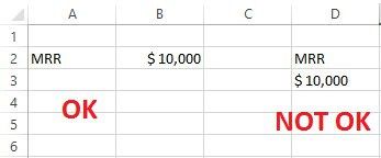
First and foremost, this formula works when you have at least two columns, where one cell has a name that defines a value vertically next or close to it.
To understand this formula, let’s divide each section of the function:
That looks pretty simple, does it? Well, it is. However, most people have a problem understanding this function.
Think it this way: when you write a VLOOKUP function, you’re trying to tell Excel: “Hey, I’m looking for this value, on this table, on this column, and I want it to be exact match.”
You just need to provide that information to Excel to make this function work. Once you understand that logic, this function gets much easier. (Believe me, I struggled with this function for a long time until I finally got it.)
One major issue with this function is that in order to this function to work, you need to have two identical values on two different tables. So make sure to have this fixed before using it, if not, it will crash.
Example: The guys from Distilled wrote a great example on how to use the VLOOKUP formula for SEO. Although this isn’t 100% relevant for marketers, it’s still quite useful.
Conclusion: If you don’t understand this function at first, don’t worry. Most people (including myself) have had problems at first with this formula. Once you understand the logic of this formula, everything will be much easier.
Useful for: Using in conjunction with other formulas, especially when that formula can end up in a “N/A” or any type of error result.
Formula: =IF(logical_test, value_if_true, value_if_false)
How it works: You start by defining a logical test, which can be anything that may end up with two results, one that verifies that test, and one that doesn’t.
Then, you specify what you want to show up when that test is true, and when it’s false.
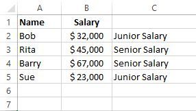
Example: Say your company has four employees, two which are senior, and two which are junior.
You consider that those that make more than $40.000 a year fall in the “Senior” category, whereas those that fall below that number fall in the “Junior” category.
In this example, the function would be:
=IF(B3>40000,”Senior Salary”,”Junior Salary”)
Conclusion: In almost all cases, you use this when you know a specific function may end up in an error.
This formula is really simple and easy to use, so you won’t have any problems learning it. There are some other related formulas for specific uses, like IFERROR, COUNTIF, AVERAGEIF, and SUMIF (see below) but they all work with the same premise as the main IF function.
Useful for: Building dynamic dashboards and tables.
Formula: =SUMIF(range, criteria, [sum_range])
How it works: The SUMIF function returns the sum of a cell range given certain criteria is met.
You start by defining the range you want to sum up, then you define the criteria to use for summing the values, and then you can optionally choose the sum range.
Example: To see the power of the SUMIF function, I highly recommend you read Annie’s post How To Use The SUMIF And SUMIFS Functions To Build Dynamic Dashboards.
Conclusion: It works exactly like the IF function, except that this function instead of returning a given value if the logical test is true or false, it returns the sum of a given range.
Useful for: Joining cells together.
Formula: =CONCATENATE(text1, [text2], …) or Cell1**&**Cell2
How it works: The CONCATENATE function and operator put together two or more text strings together.
The only difference between the CONCATENATE function and operator, is that in the first case, you use a function (that is, you need to write the whole “=CONCATENATE()”), whereas with the operator, you just use the ampersand (“&”) symbol.
Their goal is exactly the same, that is, joining strings together.
Example: Annie from Annielytics (probably the best Excel blog for marketers there is) wrote an article called 21 Real-World Examples Of Concatenating Marketing Data In Excel, in which you’ll see how useful this function is in the real world.
Conclusion: This is probably the most simple formula of the list. The only thing you need to do is select the two or more cells you want to concatenate, use either the CONCATENATE function or operator, and voila!
Useful for: Extracting data from a specific part of a given string.
Formula: =LEFT(text,num_chars), =RIGHT(text,num_chars), =MID(text, start_num, num_chars)
How it works: The LEFT and RIGHT functions work by taking an n amount of characters from the beginning (LEFT function) or end (RIGHT function) of any given string.
Both the LEFT and RIGHT functions are pretty straightforward. You start by selecting the string you’re interested in, and then you define the number of characters from the left or right of that string you want to start counting.
If you use the LEFT function, and you define you’re interested in only 5 characters, the function will select the first 5 characters of any given string.
The opposite happens with the RIGHT function. If you select 5 characters, it will select the last 5 characters from any given string.
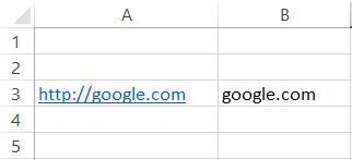
Example #1: Say you have the URL from Google, and you want to take out the “http://” from it, so you end up with the “google.com” alone. The RIGHT function would come perfect in here.
The RIGHT function would be:
RIGHT(A3, 10)
Being A3 the cell that you’re extracting the data from, and 10 the number of characters from the right you’re extracting.
On the other hand, the MID function extracts any given character from a text string starting somewhere in the middle, and continues for a set number of characters.
The MID function asks for the text to extract the data from, the starting number in the string from where you want to start the data extraction, and how many characters more you require.
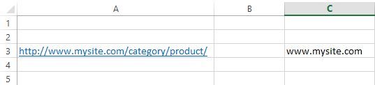
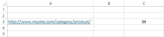
Example #2: Say you have the URL of an ecommerce site, and you just want to extract the domain name, without the “http://”, and the category and product URL. In this case, you could use the MID function to extract just the domain name.
In that case, the MID function would be:
=MID(A3, 8, 14)

Being A3 the cell where to extract the data from, 8 the number of characters to start from, and 14 the number of characters that I want to extract from the starting point given previously.
Conclusion: Although you may be scratching your head thinking in which cases you would use functions like these ones, believe me, you’ll use them more than you think.
These functions are extremely useful when put together with many other functions, like the following one.
Useful for: Specifying the starting number in the formula when you have multiple occurrences of the same character.
Formula: =FIND(find_text, within_text, [start_num])
How it works: The FIND function finds any given character or string inside another string, and tells at what position it starts in that other string.
The function starts by defining the text you want to find (which could be anything, like a number, a symbol or a word).
Then, you select the cell where that text is located. Finally, you can optionally choose the function to start an n number of characters from the LEFT of that text you are looking for.
This last part works exactly like the second parameter of the MID function.
Also, the last part is useful when there’s more than one occurrence of that text you’re looking for.
Example: Although this function is almost never used on its own, let’s say I want to know the number of characters there are until you get the “@” symbol of a list of emails.
In that case, the function would be as follows:
=FIND(“@”,B2)
Being the “@” symbol the text I’m looking for, and B2 the cell where the text is (of course, that is also valid for the whole B column).
Conclusion: This function, like most of the functions on this post, is usually used inside another function, as on its own the FIND function isn’t that useful.
More specifically, the FIND function is used in the second or third argument of the MID function (start_num, num_chars) to find a pattern from a number or cells.
Useful for: Getting the length of a string.
Formula: =LEN(find_text, within_text, [start_num])
How it works: The LEN function tells the number of characters in any given cell.
You simply select the cell you want to know the length, and that’s it.
Example: Using the example from the function #5, you have an ecommerce URL, and you want to know its length.
In that case, you would simply write “LEN()” and inside the parenthesis, you would select the cell you want to get the length from.
Conclusion: This is another simple function. Although this function is usually used together with other functions (like the IF function), it’s still a really easy and simple function to learn and use.
Useful for: Knowing where a specific value is on a given table to use into another function.
Formula: =MATCH(lookup_value, lookup_array, [match_type])
How it works: The MATCH function checks an item against a list and tells you where it appears on that list.
It works similarly to a VLOOKUP, although the MATCH function just tells in which row a specific item is, and nothing else.
This function is extremely useful, however, when you use it together with the INDEX function (see next).
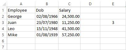
Example: Say you have a table with your employees, their day of birth, and their salary. Given that your favorite employee is Leo (because he calls “soccer” football, as it should be), you want to know where he is on that table.
In this case, the MATCH function would be:
=MATCH(“Leo”, A1:A5, 0)
Conclusion: As you have seen, the MATCH function is not that useful on itself. However, it’s really useful when is used together with the INDEX function (see below).
Useful for: Selecting one specific cell to use into another function.
Formula: =INDEX(array, row_num, [column_num])
How it works: The INDEX function gives the value of a cell located at a given array.
The INDEX function has two formulas:
The first one selects a specific row from a specific array. It can also include a specific column.
The second one selects a specific row from a reference, that is, a group of arrays. It can also include a specific column.
As I said before, this function is really useful to use it with the MATCH function to substitute the VLOOKUP function.
Example: I highly recommend you read the Excel for SEO’s guide made by the guys from Distilled and go specifically to the INDEX and MATCH part, where they give a great example on how you would use both functions together.
Conclusion: If you want to know more about the INDEX function, I recommend you read Annie’s articles on this topic.
Useful for: Selecting a group of rows and columns to use into another function.
Formula: =OFFSET(reference, rows, cols, [height], [width])
How it works: The OFFSET function works similarly to the INDEX and MATCH functions, as it returns a cell or range of cells that is a specified number of rows and columns from a cell or range of cells.
You start by selecting a reference cell, which would be “the starting cell”. From that reference cell, you select one specific cell by defining the number of rows (to the left or to the right), and the number of columns (below or above that reference cell) from the reference cell.
Up until this point, the OFFSET function works exactly like the INDEX function.
(One piece of advice: if you need a function that selects one cell from another reference cell, always use the INDEX function, as it’s more stable.)
However, this function gets interesting when you use the height and width optional values. These values work as a lasso tool, as they select a group of rows and columns from the last cell you selected.
So, this tool basically starts by selecting a reference cell, then it selects another cell from that reference cell, and it ends (optionally) by selecting a group of rows and columns from that last cell.
Example: As always, Annie Cushing has written an amazing article called Three Marketing Examples Of The OFFSET Function, in which you’ll see when you can use the OFFSET function.
Conclusion: Although the OFFSET function is useful, it’s also very unstable. Changing one single thing from the group of rows and columns selected can break a whole file, so try to use the INDEX function (alone or together with another function) whenever you can.
Are you ready to start implementing these 10 Excel function?
Then you definitely want to download the FREE guide I put together for you.
It contains all the actionable steps from this article so you can implement them whenever you want.
🎁 Free Bonus: Click here to download your bonus